Harley, Adam W., Konstantinos G. Derpanis, and Iasonas Kokkinos. “Segmentation-Aware Convolutional Networks Using Local Attention Masks.” 2017 IEEE International Conference on Computer Vision (ICCV) (2017)
Embedding을 이용한 Sementic Segmantation을 키워드로 해당 논문을 찾게 되었다. 기존의 Approach와 논문이 제안하는 Approach가 합리적으로 잘 설명되어 있고, 제안하는 식을 미분 가능하게 하여, End-to-End Learning이 가능하게 했다는 점이 인상 깊어 리뷰를 하게 되었다.
Problem Definition
기존의 CNN 연산은 사전에 정의된 Convolution Filter 크기에 따라 동일하게 연산되어, smoothing하는 효과가 내제되어 있다. 따라서 본 논문에서는 obeject의 segmentation region을 인지하고, attention을 주는 방식의 Segmentation-Aware CNN을 제안한다.
"We incorporate such masks in CNNs and replace the convolution operation with a segmentation-aware variant that allows a neuron to selectively attend to inputs coming from its own region"
Introduction
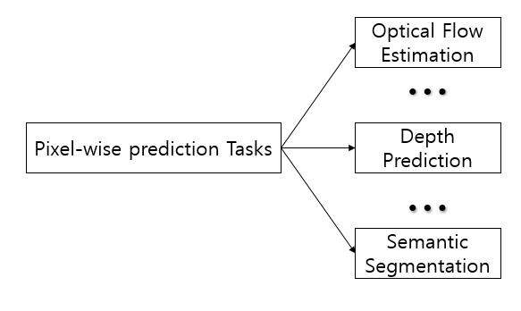
Pixel-wise prediction tasks 즉 Dense prediction 모델들은 Subsampling과 Pooling을 거치면서 1. low resolution문제와 2. smoothness 문제를 겪는다. low resolution 문제는 atrous convolution이나 upsampling 을 통해 해결하려는 접근이 있지만, 아직 smoothness 문제를 위한 연구가 상대적으로 적다. predefined convolutional filter는 다른 region 간에 spatial pooing이 되기에 smoothing되고, abstract되어 high-level task에는 적합할 수 있지만, dense prediction 문제에서는 region boundary나 motion discontinuities와 같이 activation에서 급격한 변화가 일어나는 부분에서 정확도가 떨어진다.

따라서 본 논문에서는 Figure 1.에서 볼 수 있는 것처럼 local foreground-background segmentation mask를 이미지에 더해줌으로 smoothness 문제를 해결하려고 한다.
Related work
Metric Learning의 목표는 pixel 간 혹은 region 간의 similarity를 예측하여 가장 유사한 feature를 생성하는 것이다.
이전의 approach는 SIFT, HOG와 같은 handcraft feature를 이용하였지만, matching 알고리즘이 bottleneck이 될 뿐만 아니라 pixel 단위의 matchng이기에 rotation, scale, partial occulusion과 같은 문제에 한계가 있다.
따라서 pixel의 RGB domain이 아니라 embedding domain으로 변환함으로서 rotation, scale, partial occulusion뿐만 아니라 interior appearance detail of objects에도 higher level invariance 할 수 있도록 한다.
이 embedding이 segmentation-aware feature maps을 얻기 위한 local attention masks로 사용된다.
Technical Approach
1. Learning segmentation cues

먼저 pixel 마다 segmentation embeddings을 구하는 단계이다. 즉 pixel이 같은 class인 경우에는 가깝게, 다른 class인 경우에는 먼 distance를 갖도록 학습할 수 있도록 수식화한다.
이 단계에서 pixel이 pixel간의 semantic similarity를 구할 수 있는 feature space로 맵핑시키는 embedding function을 학습해야한다.
일단 주어진 RGB image, $I$의 pixels, $p\in \Re ^{3}$ 3차원 color 벡터라고 하자. 그리고 feature space의 dimension은 $D = 64$로 선택하면, embedding function은 $f: R ^{3} \mapsto R ^{D}$이다.특히 $f(p) = e$ pixel $p$에 대한 embedding은 $e$이다.
Figure 2.는 2차원으로 간단하게 도식화한 그림이다. 임의의 pixel의 index $i, j$에 대해서 해당하는 embeddings을 $e_{i}, e_{j}$, object class labels을 $l_{i}, l_{j}$이라고 하면, 같은 class의 픽셀 쌍은 near embeddings에 다른 class의 픽셀 쌍은 far embeddings으로 최적화를 할 수 있다. 수식 (1)의 $\alpha$와 $\beta$는 각각 "near", "far"의 threshold 값이다.
pairwise loss는 식 (1)과 같다.

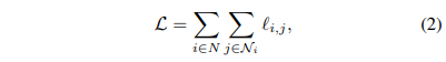
$N$ 개의 픽셀에 대하여 이미지의 모든 pairwise loss를 구하려면 $N^{2}$ 번의 연산이 필요하다. 따라서 효율적으로 sampling을 하기 위해서 index $i$에 대해서 spatial neighborhoods $j \in N_{i}$에 대해서만 계산을 한다. - 수식(2)
2. Segmentation-aware bilateral filtering

서로 다른 두 embedding 간의 거리는 같은 object class에 속하는 지, 아닌 지를 나타내는 magnitude를 의미한다. exponential distribution을 사용하여 식 (3)과 같이 확률로서 나타낼 수 있다.

기호 $m_{i, j}$는 reference 픽셀(center) $i$와 neighbor 픽셀 $j$의 foreground-background segmentation mask를 의미한다. 예를 들어 픽셀 $i$가 foreground일 때, 이웃 픽셀 $j$가 foreground일 활률 정도로 생각할 수 있겠다. 따라서 같은 픽셀에 해당하는 경우 $m_{i, i} = 1$이 된다. Figure 3.은 학습된 segmentaion mask와 intermediate embedding을 보여주고, RGB space에서 계산된 mask와 차이를 비교하는 그림이다.

input feature가 $x_{i}$라고 할 때, 수식 (4)와 같이 segmentation-aware smoothed result $y_{i}를 구할 수 있다. $k$는 index $i$로부터 spatial displacement이다. 수식 (4)는 embeddings $e^{j}$에 따라서 재미있는 special cases들이 아래와 같이 있다.
Figure 4.는 segmentation-aware bilateral filtering이 FC8의 예측값을 실제로 어떻게 sharpening하는 지 보여준다.

3. Segmentation-aware CRFs
4. Segmentation-aware Convolution
수식 (4)의 bilateral filter는 학습 가능한 task-specific filter가 아니라 non-linear sharpening mask이다. 두 장점을 다 취하기 위하여 수식 (7)과 같이 learnable parameter인 $t_{i}$를 추가한다.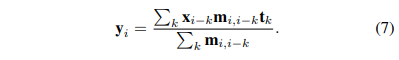
Network architecture

전반적인 network 구조이다. 처음 Embedding Network로 이미지의 싸이즈가 변화되는 layer 마다 segmentation-aware loss를 주어 학습시키고, 이를 baseline으로 사용한다. 그 후에 task-specific network를 디자인한다.
본 논문에서는 segmentic segmentaion과 optical flow 2개의 task로 성능을 평가한다.
Evaluation
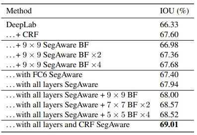
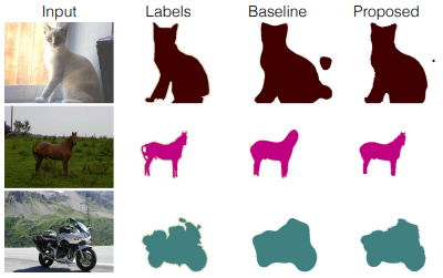
1. Semantic Segmentation


2. Optical Flow


'CV > Paper' 카테고리의 다른 글
| Instance segmentation survey (0) | 2020.03.05 |
|---|
